Motivation via Path Integral and Fresnel's Integral

In the path integral formulation of quantum mechanics, the transition amplitude between two (Heisenberg) states \(|a, t_a\rangle\) and \(|b, t_b\rangle\) is given by:

\[ \langle b,t_b|a,t_a\rangle = \int_{\mathbb{R}} \mathcal{D}x\,e^{\frac{i}{\hbar} S[x]} \]

Physically, we are considering contributions from both the classical path and quantum fluctuations around it, where the weight is determined by the exponential. Although ubiquitous, these types of integral are only conditionally convergent and ill-defined due to the oscillatory nature of the integrand. Traditional methods to overcome this problem include a Wick rotation or the \(\epsilon\)-prescription.

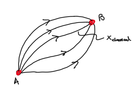
In the path integral formulation, the transition amplitude between states A and B is given by the sum of all possible paths between them.

Let's look at a simpler example — the two-dimensional Fresnel integral: \[ I = \int_{\mathbb{R}^2} dx\,dy\,e^{i(x^2 + y^2)} \]

Two evaluation methods yield different results:

Method 1: \[ I_1 = \lim_{R_x \to \infty} \lim_{R_y \to \infty} \int_{-R_x}^{R_x} dx\,e^{ix^2} \int_{-R_y}^{R_y} dy\,e^{iy^2} = \left((1+i)\sqrt{\frac{\pi}{2}}\right)^2 = i\pi \]

Method 2 (polar coordinates): \[ I_2 = 2\pi \lim_{R \to \infty} \int_0^R dr\,r\,e^{ir^2} = i\pi \lim_{R \to \infty} (1 - e^{iR^2}) \]

These methods yield conflicting results, showcasing the problem in defining such integrals.

The Picard-Lefschetz Machinery

Consider the simpler 1D case: \[ I = \int_D dx\,e^{i\phi(x)} \] with the infinite domain \(D \subseteq \mathbb{R}\) and \(\phi:\mathbb{R} \rightarrow \mathbb{R}\).

Since \(|e^{i\phi}| = 1\), this integral is conditionally convergent. The machinery proceeds in four steps:

1. Analytically continue the exponent and split into converging + oscillating factors.
2. Find steepest descent/ascent paths.
3. Verify convergence.
4. Deform the contour appropriately.

Let \(x \to z = x + iy\), hence allowing for the analytical continuation of the exponent: \[ i\phi(x) \to h(x, y) + iH(x, y) \] where \(h\) is the converging term and \(H\) oscillating.

Cauchy's theorem allows us to choose contours. We choose ones that dampen the integrand the fastest.

Consider this rather arbitrary construction: \[ \tilde{\nabla} h \cdot \tilde{\nabla} H = \partial_x h~\partial_x H + \partial_y h~\partial_y H = 0 \]

The operator \(\tilde{\nabla}\) is a modified 2D gradient operator. It behaves normally under dot products, but as a vector its parity indicates direction of flow . If you're worried about rigour, this will be the only time we use it so bear with me!

Let \(n\) be a simple saddle point. We define steepest paths: \[ \mathcal{J}_n: \tilde{\nabla}h < 0 \Rightarrow \tilde{\nabla}H = 0,\quad \mathcal{K}_n: \tilde{\nabla}h > 0 \Rightarrow \tilde{\nabla}H = 0 \] where \(\mathcal{J}_n\) is descent (Lefschetz thimble) and \(\mathcal{K}_n\) ascent. These happen to be paths where imaginary part is constant.

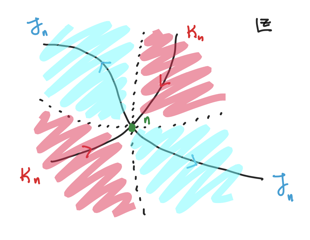
Lefschetz thimbles \(\mathcal{J}_n\) and steepest ascents \(\mathcal{K}_n\) from saddle \(n\).

A good rule of thumb is to remember that the function \(H\) finds steepest paths, while \(h\) classifies them as descent/ascent.

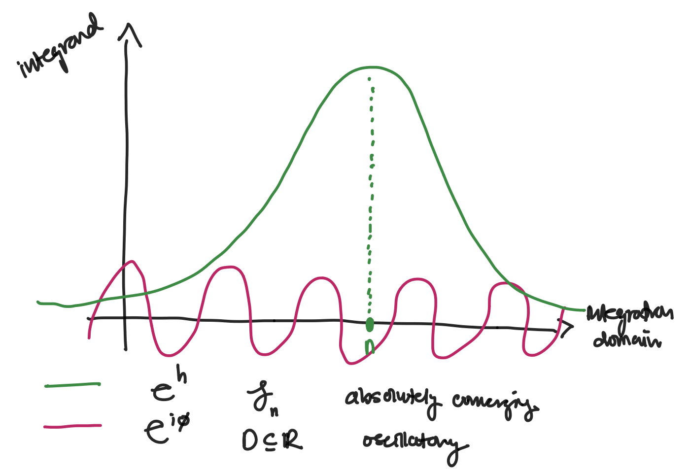
Along original contour, the integrand fluctuates. Along thimbles, integration decays as we move away from the saddle.

At this point, we have all the pieces to solve our integral. To tie it all together, we must now be able to find a Cauchy-approved deformation of the original domain such that it now passes through the saddle point \(n\) along the path of steepest descent.

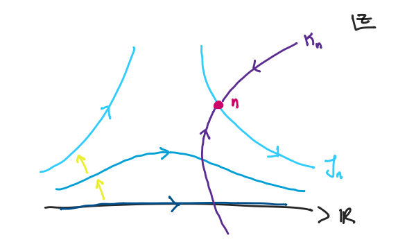
Relevant saddles are ones such that the path of steepest ascents \(\mathcal{K}_n\) intersects the original integration domain.

Imagine continuously deforming the original integration domain such that the 'direction of deformation' flows along the steepest ascent path of a saddle point. If the product of this deformation intersects a saddle point, this implies that flowing backwards in time through the initial direction of deformation is the same as the path of steepest descent from said saddle point.

The deformation theorem then implies that relevant saddle points are ones such that the path of steepest ascent \(\mathcal{K}_n\) crosses the original integration domain!

Equipped with saddles and all the steepest paths, we can finally evaluate our integral exactly along the set of Lefschetz thimbles through all relevant saddle points:

\[ I = \sum_{\sigma} n_{\sigma} e^{iH}\int_{\mathcal{J}_\sigma}dz\,e^h \]

with \(n_\sigma\) being \(\pm1\) depending on the direction integration.